
Programming with Python
Analyzing Topographic Data
Learning Objectives
- Explain what a library is, and what libraries are used for
- Load a Python library and use the tools it contains
- Read data from a file into a program
- Assign values to variables
- Select individual values and subsections from data
- Perform operations on arrays of data
- Display simple graphs
While a lot of powerful tools are built into languages like Python, even more tools exist in libraries.
In order to load the elevation data, we need to import a library called NumPy. You should use this library if you want to do fancy things with numbers (ie. math), especially if you have matrices or arrays. We can load NumPy using:
import numpyImporting a library is like pulling a toolbox out of a storage locker and placing it on your workbench, making everything inside the toolbox accessible. Python has a set of built-in functions that are always available (the tools you always have available) and libraries provide additional functionality (the specialized tools in the toolbox you only sometimes need).
Once we’ve loaded the library, we can call a function inside that library to read the data file:
numpy.loadtxt('data/topo.asc', delimiter=',')array([[ 3198.8391, 3198.123 , 3197.1584, ..., 2583.3293,
2585.4368, 2589.1079], [ 3198.3306, 3197.5242, 3196.4102, ...,
2582.6992, 2584.9167, 2587.801 ], [ 3197.9968, 3196.9197,
3195.7188, ..., 2581.8328, 2583.8159, 2586.0325], ..., [
3325.1509, 3334.7822, 3343.3154, ..., 2780.8191, 2769.3235,
2762.373 ], [ 3325.0823, 3335.0308, 3345.4963, ..., 2775.3345,
2765.7131, 2759.6555], [ 3326.6824, 3336.5305, 3348.1343, ...,
2769.7661, 2762.5242, 2756.6877]])The expression numpy.loadtxt(...) is a function call that asks Python to run the function loadtxt that belongs to the numpy library. This dotted notation, with the syntax thing.component, is used everywhere in Python to refer to parts of things.
The function call to numpy.loadtxt has two parameters: the name of the file we want to read, and the delimiter that separates values on a line. Both need to be character strings (or strings, for short) so we write them in quotes.
Within the Jupyter (iPython) notebook, pressing Shift+Enter runs the commands in the selected cell. Because we haven’t told iPython what to do with the output of numpy.loadtxt, the notebook just displays it on the screen. In this case, that output is the data we just loaded. By default, only a few rows and columns are shown (with ... to omit elements when displaying big arrays).
Our call to numpy.loadtxt read the file but didn’t save it to memory. In order to access the data, we need to assign the values to a variable. A variable is just a name that refers to an object. Python’s variables must begin with a letter and are case sensitive. We can assign a variable name to an object using =.
Let’s re-run numpy.loadtxt and assign the output to a variable name:
topo = numpy.loadtxt('data/topo.asc', delimiter=',')This command doesn’t produce any visible output. If we want to see the data, we can print the variable’s value with the command print:
print topo [[ 3198.8391 3198.123 3197.1584 ..., 2583.3293 2585.4368
2589.1079] [ 3198.3306 3197.5242 3196.4102 ..., 2582.6992
2584.9167 2587.801 ] [ 3197.9968 3196.9197 3195.7188 ...,
2581.8328 2583.8159 2586.0325] ..., [ 3325.1509 3334.7822
3343.3154 ..., 2780.8191 2769.3235 2762.373 ] [ 3325.0823
3335.0308 3345.4963 ..., 2775.3345 2765.7131 2759.6555] [
3326.6824 3336.5305 3348.1343 ..., 2769.7661 2762.5242
2756.6877]]Check your understanding
Track how variable names and values are connected after each statement in the following program:
mass = 47.5
age = 122
mass = mass * 2.0
age = age - 20
Sorting out references
What does the following program print out?
first, second = 'Grace', 'Hopper'
third, fourth = second, first
print third, fourth
Using its variable name, we can see that type of object the variable name topo is assigned to:
print type(topo) <type 'numpy.ndarray'>The function type tells us that the variable name topo currently points to an N-dimensional array created by the NumPy library. We can also get the shape of the array:
print topo.shape(500, 500)This tells us that topo has 500 rows and 500 columns. The file we imported contains elevation data (in meters, 2 degree spacing) for an area along the Front Range of Colorado, so the area that this array represents is 1 km x 1 km.
The object of type numpy.ndarray that the variable topo is assigned to contains the values of the array as well as some extra information about the array. These are the members or attributes of the object, and they describe the data in the same way an adjective describes a noun. The command topo.shape calls the shape attribute of the object with the variable name topo that describes its dimensions. We use the same dotted notation for the attributes of objects that we use for the functions inside libraries because they have the same part-and-whole relationship.
Plotting
Rasters are just big two dimensional arrays of values. In the case of DEMs, those values are elevations. It’s very hard to get a good sense of what this landscape looks like by looking directly at the data. This information is better conveyed through plots and graphics.
Data visualization deserves an entire lecture (or course) of its own, but we can explore a few features of Python’s matplotlib library here. While there is no “official” plotting library in Python, this package is the de facto standard.
We start by importing the pyplot module from the library matplotlib:
import matplotlib.pyplotWe can use the function imshow within matplotlib.pyplot to display arrays as a 2D image:
matplotlib.pyplot.imshow(topo)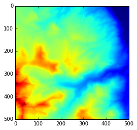
Indexing
We can access individual values in an array using an index in square brackets:
print 'elevation at the corner of topo:', topo[0,0], 'meters'elevation at the corner of topo: 3198.8391 metersprint 'elevation at some random point in topo:', topo[137,65],
'meters'elevation at some random spot in topo: 3251.1179 metersWhen referring to entries in a two dimensional array, the indices are ordered [row,column]. The expression topo[137, 65] should not surprise you but topo[0,0] might. Programming languages like Fortran and MATLAB start counting at 1 because that’s what (most) humans have done for thousands of years. Languages in the C family (including C++, Java, Perl, and Python) count from 0 because that’s simpler for computers to do. So if we have an M×N array in Python, the indices go from 0 to M-1 on the first axis (rows) and 0 to N-1 on the second (columns). In MATLAB, the same array (or matrix) would have indices that go from 1 to M and 1 to N. Zero-based indexing takes a bit of getting used to, but one way to remember the rule is that the index is how many steps we have to take from the start to get to the item we want.
Python also allows for negative indices to refer to the position of elements with respect to the end of each axis. An index of -1 refer to the last item in a list, -2 is the second to last, and so on. Since index [0,0] is the upper left corner of an array, index [-1,-1] therefore the lower right corner of the array:
print topo[-1,-1]2756.6877Check your understanding
Draw diagrams showing how variable names and values are connected after each statement in the following program:
mass = 47.5
age = 122
mass = mass * 2.0
age = age - 20
Sorting out references
What does the following program print out?
first, second = 'Grace', 'Hopper'
third, fourth = second, first
print third, fourth
Slicing
A command like topo[0,0] selects a single element in the array topo. Indices can also be used to slice sections of the array. For example, we can select the top left quarter of the array like this:
print topo[0:5, 0:5][[ 3198.8391 3198.123 3197.1584 3196.2017 3193.8813] [
3198.3306 3197.5242 3196.4102 3194.7559 3191.9763] [ 3197.9968
3196.9197 3195.7188 3193.3855 3190.5371] [ 3198.054 3196.7031
3194.9573 3192.4451 3189.5288] [ 3198.3289 3196.9111 3195.335
3192.7874 3190.0085]]
The slice [0:5] means “Start at index 0 and go along the axis up to, but not including, index 5”.
We don’t need to include the upper or lower bound of the slice if we want to go all the way to the edge. If we don’t include the lower bound, Python uses 0 by default; if we don’t include the upper bound, the slice runs to the end of the axis. If we don’t include either (i.e., if we just use ‘:’), the slice includes everything:
print topo[:len(topo)/2, len(topo)/2:][[ 3008.1116 3012.2922 3015.3018 ..., 2583.3293 2585.4368
2589.1079] [ 3009.9558 3014.0007 3016.5647 ..., 2582.6992
2584.9167 2587.801 ] [ 3010.8604 3014.1228 3016.7412 ...,
2581.8328 2583.8159 2586.0325] ..., [ 3370.0918 3368.5371
3366.7148 ..., 2687.8396 2682.4326 2676.8521] [ 3370.478
3368.7561 3366.8923 ..., 2685.9941 2681.2888 2676.9924] [
3371.2021 3369.3376 3367.3677 ..., 2687.7014 2685.5146
2683.1936]]Point elevations
Use indexing to answer the following questions and check your answers against the data visualization:
- Is the NW corner of the region higher than the SW corner? What’s the elevation difference?
- What’s the elevation difference between the NE corner and the SE corner?
- What’s the elevation at the center of the region shown in the array?
Slicing strings
Indexing and slicing behave the same way for any type of sequence, including numpy arrays, lists, and strings. Create a new variable called text and assign it the string “The quick brown fox jumped over the lazy dog.” (note the capitalization and punctuation in each sentence, and include the quotes so Python recognizes it as a string). Then use slicing and the print statement to create these frases:
- the lazy dog.
- The fox jumped over the dog
- The lazy fox jumped over the quick brown dog.
Plotting smaller regions
Use the function imshow from matplotlib.pyplot to make one plot showing the northern half of the region and another plot showing the southern half.
Then try making four separate plots showing each quarter of the region separately.
Non-square arrays
We’ve been using len(topo)/2 as both the row and column indices of the center point in the array topo. This doesn’t work with an array that’s not square (has different height and width).
Take a (small) slice of the array
topoand assign it to a new variable. Make this new array have a height longer than its width, and make both the height and width even numbers (4 x 6 is a good size).Access the center point of your new array. Write the indices using variables, not numbers (ie. don’t write
t[2,3]) (Hint:topo.shapegives the number of rows and columns intopo. The functionlen(topo)returns the length of the longest axis. Instead of usinglen(), assign the output ofshapeto a variable and use indexing). Are you really pointing to the center of your array? How far off are you?
Odd-sized arrays
Both the array topo and the one you created above have even numbers of rows and columns. In that case, the output of width/2 and height/2 were both whole numbers (and therefore valid indices). Mysteriously, len(topo)/2 would work as an index even if the array topo had odd numbers of rows and columns. Let’s test it out!
Take a second slice of
topothat is one row and column larger than the one you made previously. Check its shape and print the value at the center of the array using indices likewidth/2andheight/2. Does this work? Should this work?Compare the actual indices of the center point of this array and the indices you would calculate by dividing its width and height by 2. Is division in Python behaving like division in the real world? (Hint: If an array has a width and height that are odd numbers, what should the value of
width/2be?).Test the behavior of division (using
/) in Python by trying various even and odd whole numbers and decimals as both the nominator and denominator.
Numerical operations on arrays
We can perform basic mathematical operations on each individual element of a NumPy array. We can create a new array with elevations in feet:
topo_in_feet = topo * 3.2808
print 'Elevation in meters:', topo[0,0]
print 'Elevation in feet:', topo_in_feet[0,0]
Elevation in meters: 3198.8391
Elevation in feet: 10494.7513193Arrays of the same size can be used together in arithmatic operations:
double_topo = topo + topo
print 'Double topo:', double_topo[0,0], 'meters'
Double topo: 6397.6782 metersWe can also perform statistical operations on arrays:
print 'Mean elevation:', topo.mean(), 'meters'Mean elevation: 3153.62166407 metersNumPy arrays have many other useful methods:
print 'Highest elevation:', topo.max(), 'meters'
print 'Lowest elevation:', topo.min(), 'meters'
Highest elevation: 3831.2617 meters
Lowest elevation: 2565.0293 metersWe can also call methods on slices of the array:
half_len = int(len(topo) / 2)

print 'Highest elevation of NW quarter:', topo[:half_len,
:half_len].max(), 'meters'

print 'Highest elevation of SE quarter:', topo[half_len:,
half_len:].max(), 'meters'
Highest elevation of NW quarter: 3600.709 meters
Highest elevation of SE quarter: 3575.3262 metersMethods can also be used along individual axes (rows or columns) of an array. If we want to see how the mean elevation changes with longitude (E-W), we can use the method along axis=0:
print topo.mean(axis=0) To see how the mean elevation changes with latitude (N-S), we can use axis=1:
print topo.mean(axis=1) Plotting, take two
It’s hard to get a sense of how the topography changes across the landscape from these big tables of numbers. A simpler way to display this information is with line plots.
We are again going to use the matplotlib package for data visualization. Since we imported the matplotlib.pyplot library once already, those tools are available and can be called within Python. As a review, though, we are going to write every step needed to load and plot the data.
We use the function plot to create two basic line plots of the topography:
import numpy as np
import matplotlib.pyplot as plt
%matplotlib inline

topo = np.loadtxt('data/topo.asc', delimiter=',')

plt.plot(topo[0,:])
plt.title('Topographic profile, northern edge')
plt.ylabel('Elevation (m)')
plt.xlabel('<-- West    East -->')
plt.show()

plt.plot(topo[-1,:], 'r--')
plt.title('Topographic profile, southern edge')
plt.ylabel('Elevation (m)')
plt.xlabel('<-- West    East -->')
plt.show() 

To better compare these profiles, we can plot them as separate lines in a single figure using the argument hold=True, This will force all subsequent calls to plt.plot to use the same axes (until it reaches plt.show()). The argument label= holds the label that will appear in the legend.
import numpy as np import matplotlib.pyplot as plt
%matplotlib inline

topo = np.loadtxt('data/topo.asc', delimiter=',')

plt.plot(topo[0,:], hold=True, label='North')

plt.plot(topo[-1,:], 'r--', label='South')

plt.plot(topo[len(topo)/2,:], 'g:', linewidth=3, label='Mid')

plt.title('Topographic profiles')
plt.ylabel('Elevation (m)')
plt.xlabel('<-- West    East -->')
plt.legend(loc = 'lower left')

plt.show() 
Make your own plots
Create three separate plots showing how the maximum (numpy.max()), minimum (numpy.min()), and mean (numpy.mean()) elevation changes with longitude. Label the axes and include a title for each of the plots (Hint: use axis=0).
Convert the separate plots into a single plot that includes all three statistics (using hold=True). Create a legend.
Subplots
We often want to arrange separate plots in layouts with multiple rows and columns. The script below uses subplots to show the elevation profile at the western edge, the mid longitude, and eastern edge of the region. Subplots can be a little weird because they require the axes to be defined before plotting. Type (don’t copy-past!) the code below to get a sense of how it works.
This script uses a number of new commands. The function plt.figure() creates a space into which we will place the three plots. The parameter figsize tells Python how big to make this space. Each subplot is placed into the figure using the subplot command. The subplot command takes 3 parameters: the first denotes the total number of rows of subplots in the figure, the second is the total number of columns of subplots in the figure, and the final parameters identifies the position of the subplot in the grid. The axes of each subplot are called with different variable (axes1, axes2, axes3, axes4). Once a subplot is created, the axes can be labeled using the set_xlabel() (or set_ylabel()) method. plt.show() is called after the entire figure is set up.
import numpy as np import matplotlib.pyplot as plt
%matplotlib inline

topo = np.loadtxt('data/topo.asc', delimiter=',')

fig = plt.figure(figsize=(16.0, 3.0))

axes1 = fig.add_subplot(1,3,1)
axes2 = fig.add_subplot(1,3,2)
axes3 = fig.add_subplot(1,3,3)

axes1.plot(topo[:,0])
axes1.set_ylim([2500,3900])
axes1.set_ylabel('Elevation (m)')
axes1.set_xlabel('<-- N   S -->')
axes1.set_title('West')

axes2.plot(topo[:,len(topo)/2])
axes2.set_ylim([2500,3900])
axes2.set_xlabel('<-- N   S -->')
axes2.set_title('Mid')

axes3.plot(topo[:,-1])
axes3.set_ylim([2500,3900])
axes3.set_xlabel('<--N   S -->')
axes3.set_title('East')

plt.show(fig)
Subplots of DEMs
Make a 2x2 grid of subplots that use the function imshow to display each quarter of the dataset (ie. split down the middle in both x and y).
- Don’t label axes or add a colorbar. It can be tricky to do this with subplots.
- To set the range of colors for one subplot, include the arguments
vminandvmaxinimshowlike this:
vmin = topo.min()
vmax = topo.max()

plt.imshow(topo, vmin=vmin, vmax=vmax)